PhasePlane | MathModel.uz

5.6-bo'lim: Faza tekisligi

Differensial tenglamalar sistemasini haqiqiy echishga kirishishdan oldin biz ko'rib chiqishimiz kerak bo'lgan bitta mavzu bor. Bu har doim ham differentsial tenglamalar sinfida o'qitilmaydigan mavzu, ammo agar siz u o'qitiladigan kursda bo'lsangiz, unga tayyor bo'lishingiz uchun uni yoritishimiz kerak.

Umumiy bir hil tizimdan boshlaylik,

\[\begin{equation}\vec x' = A\vec x\label{eq:eq1}\end{equation}\]

E'tibor bering

\[\vec x = \vec 0\]

differensial tenglamalar sistemasining yechimidir. Biz so'ramoqchi bo'lgan narsa, $t$ o'sishi bilan tizimning boshqa echimlari ushbu yechimga yaqinlashadimi yoki ular bu yechimdan uzoqlashadimi? Oldingi maqolada muvozanat yechimlarini tasniflaganimizda shunga o'xshash ishni qildik bo'limi. Aslida, biz bu erda qilayotgan narsa bu g'oyaning differentsial tenglamalar sistemalariga kengaytmasidir.

$\vec x = \vec 0$ yechimi an deb ataladi muvozanatli yechim tizimi uchun. Yagona differensial tenglamalarda bo'lgani kabi, muvozanatli echimlar ham shunday echimlardir

\[A\vec x = \vec 0\]

Biz $A$ yagona bo'lmagan matritsa deb faraz qilamiz va shuning uchun faqat bitta yechim bo'ladi,

\[\vec x = \vec 0\]

va shuning uchun biz faqat bitta muvozanat yechimiga ega bo'lamiz.

Yagona differensial tenglama holatida biz $y$ qiymatlarini tanlash va $y'$ qiymatlarini aniqlash uchun ularni $f(y)$ funksiyasiga ulashdan boshlaganimizni eslaymiz. Keyin biz ushbu qiymatlardan $y$ ning ma'lum bir qiymatida yechimning tangenslarini chizish uchun foydalandik. Shundan kelib chiqib, biz ba'zi yechimlarning eskizini chizishimiz va bu ma'lumotlardan muvozanatli echimlarni tasniflash uchun foydalanishimiz mumkin.

Biz bu erda shunga o'xshash narsani qilmoqchimiz, lekin u ham biroz boshqacha bo'ladi. Birinchidan, biz o'zimizni $2 \times 2$ ishi bilan cheklaymiz. Shunday qilib, biz shakl tizimlarini ko'rib chiqamiz,

\[\begin{array}{*{20}{c}}\begin{aligned}{{x'}_1} & = a{x_1} + b{x_2}\\ {{x'}_2} & = c{x_1} + d{x_2}\end{aligned}&{\hspace{0.25in} \Rightarrow \hspace{0.25in}\hspace{0.25in}\vec x' = \left( {\begin{array}{*{20}{c}}a&b\\c&d\end{array}} \right)\vec x}\end{array}\]

Ushbu tizimning echimlari quyidagi shaklda bo'ladi:

\[\vec x = \left( {\begin{array}{*{20}{c}}{{x_1}\left( t \right)}\\{{x_2}\left( t \right)}\end{array}} \right)\]

va bizning yagona muvozanat yechimimiz bo'ladi,

\[\vec x = \left( {\begin{array}{*{20}{c}}0\\0\end{array}} \right)\]

Yagona differensial tenglama holatida biz $y(t)$ yechimini chiza oldik. y-t tekislang va haqiqiy echimlarni ko'ring. Biroq, bu holda bu biroz qiyin bo'ladi, chunki bizning echimlarimiz aslida vektordir. Bu erda biz nima qilmoqchimiz, tizim echimlarini ${x_1}\,{x_2}$ tekisligidagi nuqtalar deb o'ylash va bu nuqtalarni chizish. Bizning muvozanat yechimimiz ${x_1}\,{x_2}$ kelib chiqishiga mos keladi. samolyot va ${x_1}\,{x_2}$ tekisligi deyiladi faza tekisligi.

Fazalar tekisligida yechimni chizish uchun biz $t$ qiymatlarini tanlashimiz va ularni yechimga ulashimiz mumkin. Bu bizga ${x_1}\,{x_2}$ yoki faza tekisligida biz chiza oladigan nuqtani beradi. Buni $t$ ning ko'p qiymatlari uchun qilish, keyin bizga yechim fazalar tekisligida nima qilishining eskizini beradi. Fazalar tekisligidagi ma'lum bir yechimning eskizi deyiladi traektoriya yechimdan. Eritmaning traektoriyasini chizganimizdan so'ng, $t$ ortishi bilan yechim muvozanat yechimiga yaqinlashadimi yoki yo'qmi, deb so'rashimiz mumkin.

Biz qo'lda echimlarsiz traektoriyalarni chizish imkoniyatiga ega bo'lishni xohlaymiz. Buni amalga oshirishning bir necha yo'li mavjud. Biz ulardan birini bu erda ko'rib chiqamiz, ikkinchisini esa keyingi ikki bo'limda ko'rib chiqamiz.

Traektoriyalar eskizini olishning usullaridan biri bu biz muvozanat yechimlarini birinchi marta ko'rganimizda qilgan ishimizga o'xshash ishni qilishdir. Biz $\vec x$ qiymatlarini tanlashimiz mumkin (esda tutingki, ular fazalar tekisligidagi nuqtalar bo'ladi) va $A\vec x$ ni hisoblashimiz mumkin. Bu $\vec x'$ at ma'lum bir yechimni ifodalovchi vektorni beradi. Yagona differentsial tenglamada bo'lgani kabi, bu vektor o'sha nuqtada traektoriyaga tegib turadi. Biz bir nechta tangens vektorlarini chizamiz va keyin traektoriyalarni chizamiz.

Bu ularni bajarishning juda mehnat talab qiladigan usuli va umuman ularni amalga oshirishning usuli emas. Biroq, bu hech qanday yechim ishini qilmasdan traektoriyalarni olishning bir usuli. Bizga faqat differentsial tenglamalar sistemasi kerak. Keling, bir misolni tez ko'rib chiqaylik.

1-misol Tizim uchun ba'zi traektoriyalarni chizing, \[\begin{array}{*{20}{c}}\begin{aligned}{{x'}_1} & = {x_1} + 2{x_2}\\ {{x'}_2} & = 3{x_1} + 2{x_2}\end{aligned}&{\hspace{0.25in} \Rightarrow \hspace{0.25in}\vec x' = \left( {\begin{array}{*{20}{c}}1&2\\3&2\end{array}} \right)\vec x}\end{array}\]

Yechim

Shunday qilib, biz qilishimiz kerak bo'lgan narsa - fazalar tekisligidagi ba'zi nuqtalarni tanlash, ularni tizimning o'ng tomoniga ulang. Biz buni bir necha nuqta uchun qilamiz.

\[\begin{align*}\vec x & = \left( {\begin{array}{*{20}{c}}{ - 1}\\1\end{array}} \right) & \Rightarrow \hspace{0.25in}\vec x'& = \left( {\begin{array}{*{20}{c}}1&2\\3&2\end{array}} \right)\left( {\begin{array}{*{20}{c}}{ - 1}\\1\end{array}} \right) = \left( {\begin{array}{*{20}{c}}1\\{ - 1}\end{array}} \right)\\ \vec x & = \left( {\begin{array}{*{20}{c}}2\\0\end{array}} \right) & \Rightarrow \hspace{0.25in}\vec x' & = \left( {\begin{array}{*{20}{c}}1&2\\3&2\end{array}} \right)\left( {\begin{array}{*{20}{c}}2\\0\end{array}} \right) = \left( {\begin{array}{*{20}{c}}2\\6\end{array}} \right)\hspace{0.25in}\\ \vec x & = \left( {\begin{array}{*{20}{c}}{ - 3}\\{ - 2}\end{array}} \right) & \Rightarrow \hspace{0.25in}\vec x' & = \left( {\begin{array}{*{20}{c}}1&2\\3&2\end{array}} \right)\left( {\begin{array}{*{20}{c}}{ - 3}\\{ - 2}\end{array}} \right) = \left( {\begin{array}{*{20}{c}}{ - 7}\\{ - 13}\end{array}} \right)\hspace{0.25in}\end{align*}\]

Xo'sh, bu bizga nimani anglatadi? Xo'sh, fazalar tekisligidagi $\left( { - 1,1} \right)$ nuqtasida $\left\langle {1, - 1} \right\rangle $ yo'nalishiga ishora qiluvchi vektor bo'ladi. $\left( {2,0} \right)$ nuqtasida $\left\langle {2,6} \right\rangle $ yo'nalishiga ishora qiluvchi vektor bo'ladi. $\left( { - 3, - 2} \right)$ nuqtasida $\left\langle { - 7, - 13} \right\rangle $ yo'nalishiga ishora qiluvchi vektor bo'ladi.

Buni fazalar tekisligidagi ko'p sonli nuqtalar uchun bajarish vektorlarning quyidagi eskizini beradi.

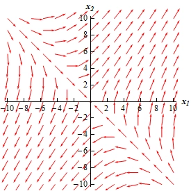
$A graph with domain $-10 \le x_{1} \le 10$ and range $-10 \le x_{2} \le 10$. This graph has a vast number of arrows on it. In the 1st quadrant the arrows all point generally towards the upper right corner and make approximately a 45 degree angle with the horizon. In the 3rd quadrant all the arrows all point generally towards the lower left corner and make approximately a 45 degree angle with the horizon. In the 2nd quadrant along an imaginary line y=-x (not shown) are a series of arrows that would fall on this line all pointing directly at the origin. Arrows that start just above this line all generally follow the same directly but are not pointed slightly to the right of the origin. As we move away from the line (still above it) the arrows start to point more directly into the 1st quadrant and by time we reach the $x_{2}$-axis the arrows are starting to look like the arrows that are in the 1st quadrant. Arrows that start just below the imaginary line all generally follow the same directly but are not pointed slightly to the left of the origin. As we move away from the line (still below it) the arrows start to point more directly into the 3rd quadrant and by time we reach the $x_{1}$-axis the arrows are starting to look like the arrows that are in the 3rd quadrant. In the 4th quadrant the arrows are similar to those in the 2nd quadrant. Along an imaginary line (not shown) y = -x arrows point directly towards the origin. Arrows that start just above this line all generally follow the same directly but are not pointed slightly to the right of the origin. As we move away from the line (still above it) the arrows start to point more directly into the 1st quadrant and by time we reach the $x_{1}$-axis the arrows are starting to look like the arrows that are in the 1st quadrant. Arrows that start just below the imaginary line all generally follow the same directly but are not pointed slightly to the left of the origin. As we move away from the line (still below it) the arrows start to point more directly into the 3rd quadrant and by time we reach the $x_{2}$-axis the arrows are starting to look like the arrows that are in the 3rd quadrant.$

Endi biz qilishimiz kerak bo'lgan narsa - ba'zi traektoriyalarda eskiz. Buni amalga oshirish uchun yuqoridagi eskizdagi vektorlar traektoriyalarga tegishini yodda tutishimiz kerak. Shuningdek, vektorlar yo‘nalishi $t$ ortishi bilan traektoriya yo‘nalishini beradi, shuning uchun biz traektoriyalarga o‘qlarni qo‘shish orqali yechimning vaqtga bog‘liqligini ko‘rsatishimiz mumkin.

Buni bajarish quyidagi eskizni beradi.

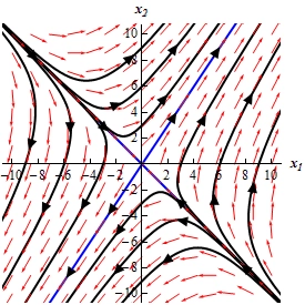
$A graph with domain $-10 \le x_{1} \le 10$ and range $-10 \le x_{2} \le 10$. This graph has a vast number of arrows on it. This graph has exactly the same set of arrows as the previous graph. To avoid making this alt text too long we will not describe those again here. Also on the graph are a series of trajectories. First, there are two lines given by approximately y=-x and y=3/2x. Along the y=-x line are arrow heads that point towards the origin. Along the y=3/2x line are arrow heads pointing away from the origin. These two lines form a giant “X” that basically divide the graph into 4 regions with three trajectories in it. In the upper region trajectories start almost on top of the y=-x line (in the 2nd quadrant) and have arrow heads again pointing in towards the origin. At approximately equal distances along this line the trajectories break off the y=-x line and follow the arrows into the 1st quadrant and end up as lines parallel to the y=3/2x line in the 1st quadrant with arrow heads on them pointing towards the upper right corner. In the left region trajectories behave similar to those in the upper region. They start following the y=-x line in the 2nd quadrant and then at approximately equal distances along the y=-x line the break off and following the arrows flow into the 3rd quadrant and end point parallel to the y=3/2x line with arrow heads on them pointing towards the lower left corner. The bottom and right regions of the “X” are basically a mirror image of the upper/left regions. Trajectories start out following the y=-x line in the 4th quadrant and then break off and flow away from the y=-x line. In the right region they flow up into the 1st quadrant ending up parallel to the y=3/2x line there with arrow heads pointing to the upper right corner. In the bottom region the flow into the 3rd quadrant and end up parallel to the y=3/2x line there with arrow heads point to the lower left corner.$

Ushbu eskiz deyiladi fazali portret. Odatda fazali portretlar faqat yechimlarning traektoriyalarini o'z ichiga oladi va vektorlarni emas. Ushbu nuqtani tashkil etuvchi barcha bosqichli portretlarimiz faqat traektoriyalarni o'z ichiga oladi.

Bunday holda, yechimlarning ko'pchiligi muvozanatli eritmadan uzoqlasha boshlaydi, keyin $t$ o'sishni boshlaganda, ular muvozanat yechimiga qarab harakatlanadi va oxir-oqibat yana muvozanat eritmasidan uzoqlasha boshlaydi.

Bir oz boshqacha xatti-harakatlarga ega bo'lgan to'rtta echim borga o'xshaydi. Eritmalarning ikkitasi muvozanat eritmasidan (yoki hech bo'lmaganda) boshlanadi va so'ngra undan to'g'ridan-to'g'ri uzoqlashadi, qolgan ikkita yechim esa muvozanat eritmasidan uzoqlashadi va keyin to'g'ridan-to'g'ri muvozanat eritmasi tomon harakatlanadi.

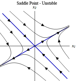
Bunday hollarda biz muvozanat nuqtasini a deb ataymiz egar nuqtasi va bu holatda muvozanat nuqtasi deb ataymiz beqaror chunki $t$ oshgani sayin ikkitadan tashqari barcha echimlar undan uzoqlashadi.

Yuqorida aytib o'tganimizdek, bu biz traektoriyalarni chizishimiz uchun umuman yo'l emas. Traektoriyalarni olish uchun bizga faqat $A$ matritsasining xos qiymatlari va xos vektorlari kerak bo'ladi. Tizimlarni hal qilishda buni qanday qilishni keyingi ikki bo'limda ko'rib chiqamiz.

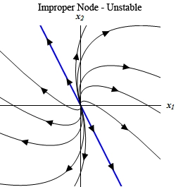
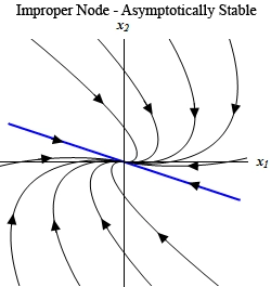
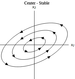
Bu erda yana bir nechta bosqichli portretlar mavjud, shuning uchun siz bir nechta mumkin bo'lgan misollarni ko'rishingiz mumkin. Haqiqatan ham, biz keyingi bo'limlar davomida ulardan bir nechtasini yaratamiz.

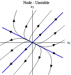
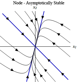
$This graph has no domain or range specified. The horizontal axis is labeled $x_{1}$ and the vertical axis is labeled $x_{2}$. The graph is labeled “Node – Unstable”. There are two lines with equations of approximately y=x and y=-3/5x on the graph. Each of these lines have arrow heads on them pointing away from the origin and divide the graph in a giant “X”. In the upper and right region of the “X” trajectories start at the origin and flow along the y=-3/5x line and at approximately equal distances along the line the break away and flow into the 1st quadrant and move out of the 1st quadrant parallel to the y=x line. They all have arrow heads on them indicating this direction of motion. In the bottom and left region of the “X” trajectories again start at the origin and flow along the y=-3/5x line and at approximately equal distances along the line the break away and flow into the 3rd quadrant and move out of the 3rd quadrant parallel to the y=x line. They all have arrow heads on them indicating this direction of motion.$ $This graph has no domain or range specified. The horizontal axis is labeled $x_{1}$ and the vertical axis is labeled $x_{2}$. The graph is labeled “Node – Asymptotically Stable”. There are two lines with equations of approximately y=5/3x and y=-x on the graph. Each of these lines have arrow heads on them pointing towards the origin and divide the graph in a giant “X”. In the upper and left region of the “X” trajectories start in the 2nd quadrant (for the upper region) and in the 3rd quadrant (for the left region) and flow down and to the right basically parallel to the y=-x line. As they get near the y=5/3x line they bend in towards that line and follow that line into the origin. They all have arrow heads on them indicating this direction of motion. In the upper and right region of the “X” trajectories start in the 1st quadrant (for the right region) and in the 4th quadrant (for the bottom region) and flow up and to the left basically parallel to the y=-x line. As they get near the y=5/3x line they bend in towards that line and follow that line into the origin. They all have arrow heads on them indicating this direction of motion.$

$This graph has no domain or range specified. The horizontal axis is labeled $x_{1}$ and the vertical axis is labeled $x_{2}$. The graph is labeled “Improper Node –Unstable”. There is a line with equation of approximately y=-5/3x on the graph with arrow heads on it pointing away from the origin. Trajectories to the right this line all start at the origin and move away from the origin into the 2nd quadrant. Trajectories, at approximately equal distances, then bend around and move into the 1st quadrant. They continue to bend around and move into the 4th quadrant and exit flow out the bottom right corner of the graph basically parallel to the line. Trajectories to the left this line all start at the origin and move away from the origin into the 4th quadrant. Trajectories, at approximately equal distances, then bend around and move into the 3rd quadrant. They continue to bend around and move into the 2nd quadrant and exit flow out the upper left corner of the graph basically parallel to the line.$ $This graph has no domain or range specified. The horizontal axis is labeled $x_{1}$ and the vertical axis is labeled $x_{2}$. The graph is labeled “Improper Node – Asymptotically Stable”. There is a line with equation of approximately y=-3/5x on the graph with arrow heads on it pointing into the origin. Trajectories above this line all start at the upper part of the graph (in the 1st and 2nd quadrant) and flow down and to the right. Those that start near the y=-3/5x line in the 2nd quadrant are nearly parallel to the line. As trajectories move into the 1st quadrant they are not quite parallel to the line. As the trajectories near the $x_{1}$ axis they bend around and move into the 4th quadrant and start to follow the line into the origin. Trajectories below this line all start at the lower part of the graph (in the 3rd and 4th quadrant) and flow up and to the left. Those that start near the y=-3/5x line in the 2nd quadrant are nearly parallel to the line. As trajectories move into the 3rd quadrant they are not quite parallel to the line. As the trajectories near the $x_{1}$ axis they bend around and move into the 2nd quadrant and start to follow the line into the origin.$

$This graph has no domain or range specified. The horizontal axis is labeled $x_{1}$ and the vertical axis is labeled $x_{2}$. The graph is labeled “Saddle Point –Unstable”. There are two lines with equations of approximately y=2/3x (with arrow heads pointing away from the origin) and y=-x (with arrow heads point towards the origin) on the graph. The lines divide the graph in a giant “X”. In the upper and left region of the “X” trajectories start in the 2nd quadrant and flow down basically parallel to the y=-x line. As they near the y=2/3x line the bend to the right (for those in the upper region) and to the left (for those in the left region) and follow the y=2/3x line out away from the origin. Arrow heads are on the trajectories indicating this direction. In the lower and right region of the “X” trajectories start in the 1st quadrant and flow up basically parallel to the y=-x line. As they near the y=2/3x line the bend to the right (for those in the right region) and to the left (for those in the bottom region) and follow the y=2/3x line out away from the origin. Arrow heads are on the trajectories indicating this direction.$ $This graph has no domain or range specified. The horizontal axis is labeled $x_{1}$ and the vertical axis is labeled $x_{2}$. The graph is labeled “Center –Stable”. The trajectories in this graph are three ellipses that are centered on the origin and “angled” so that their major axis (i.e. the long part of the ellipse) are in the 1st and 3rd quadrants. There are arrow heads on the ellipses indicating they are traced out in a counter clockwise direction.$

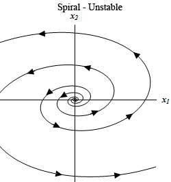
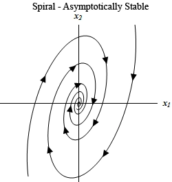
$This graph has no domain or range specified. The horizontal axis is labeled $x_{1}$ and the vertical axis is labeled $x_{2}$. The graph is labeled “Spiral –Unstable”. There are two trajectories on this graph. Each is a spiral that starts at the origin and rotates out away from the origin in a counter clockwise manner.$ $This graph has no domain or range specified. The horizontal axis is labeled $x_{1}$ and the vertical axis is labeled $x_{2}$. The graph is labeled “Spiral –Unstable”. There are two trajectories on this graph. Each is a spiral that starts at the outer edges (one starts at upper right corner and the other starts at the bottom left corner) and rotates into the origin in a clockwise manner.$

Bu erda barcha mumkin bo'lgan bosqichli portretlar ko'rsatilmagan. Bular sizga ba'zi imkoniyatlarni ko'rsatish uchun. O'qlar yo'nalishiga qarab, bir nechta turlar asimptotik barqaror yoki beqaror bo'lishi mumkinligini unutmang.

O'rtasidagi farqga e'tibor bering barqaror va asimptotik barqaror. Asimptotik barqaror tugun yoki spiralda barcha traektoriyalar muvozanat nuqtasiga qarab harakatlanadi. t ortadi, holbuki markaz (har doim barqaror) traektoriya faqat muvozanat nuqtasi atrofida harakat qiladi, lekin hech qachon unga qarab harakat qilmaydi.